10 Excel 2013 Advanced Formulas and Functions: Power-Up Your Spreadsheets with Pro-Level Shortcuts

Struggling with complex calculations that require multiple steps? Array formulas in Excel 2013 let you perform advanced math—like averages, sums, or conditional logic—all within a single cell. No more cluttering your spreadsheet with helper columns or nested IF statements.

To use them, press Ctrl+Shift+Enter (not just Enter) to activate the formula. For example, {=SUM(A1:A10*B1:B10>50)} multiplies values in range A1:A10 by B1:B10 only if B1:B10 exceeds 50, then sums the results. This is perfect for financial modeling, where you might need to calculate weighted averages or dynamic ranges without restructuring your data.

Accountants, analysts, and data-driven professionals will love this for streamlining workflows. Just remember: array formulas recalculate automatically when referenced data changes, making them a zero-config power tool for dynamic spreadsheets. ✨

Tired of VLOOKUP breaking when your data rearranges? The INDEX-MATCH duo is the Swiss Army knife of Excel lookups—flexible enough to handle both vertical and horizontal searches while avoiding the infamous #N/A errors that plague VLOOKUP in messy datasets.

Here’s how it works: INDEX retrieves a value from a range based on row and column positions, while MATCH locates the position of a lookup value. Combined, they let you pull data from anywhere—even non-contiguous ranges—without restructuring your sheet. For example, =INDEX(B2:B100, MATCH("Apple", A2:A100, 0)) finds "Apple" in column A and returns its value from column B, but swap the columns and it works just as well. ⚡

This is the go-to for database-style tasks like inventory tracking, sales reporting, or merging datasets where VLOOKUP’s limitations would otherwise force manual workarounds. Perfect for analysts who need reliability over rigid column structures.

Tired of manually filtering data before summing values? SUMIFS and SUMIF let you add conditional logic directly into your calculations—no extra steps required. These functions are game-changers for scenarios where you need to aggregate data based on multiple criteria, like summing sales for products in a specific region and price range.

SUMIF handles one condition (e.g., sum values where "Region = West"), while SUMIFS lets you stack up to 127 criteria (e.g., sum sales where "Region = West" and "Price > $50" and "Date > 1/1/2023"). Both work seamlessly with text, numbers, or dates, and they’re faster than manual filtering—ideal for inventory tracking or dynamic dashboards. The syntax is straightforward once you get past the comma-heavy setup.

Small business owners and analysts will love these for automating repetitive reports, while inventory managers can use them to track stock levels by category and location—all without touching a single filter button. ✨

Tired of messy text strings ruining your data exports or reports? TEXTJOIN and TRIM in Excel 2013 are your secret weapons for cleaning and combining text efficiently—without manual copy-pasting or error-prone concatenation.

TEXTJOIN lets you merge text from multiple cells with a custom delimiter (like commas or semicolons), while TRIM strips away invisible spaces that often sneak into imported data. For example, =TEXTJOIN(", ", TRUE, A1:A10) combines cells A1 through A10 with spaces between entries, and =TRIM(B1) removes extra spaces from cell B1. Together, they’re perfect for preparing CSV exports or merging data from different sources.

Accountants, data analysts, and anyone dealing with imported datasets will love these functions for their precision and speed. They’re especially useful when you need to combine product names, customer lists, or any text-heavy data without headaches. ✨

Tired of manually adjusting dates for payroll deadlines or project milestones? EDATE and EOMONTH in Excel 2013 automate these tasks with precision, saving you time and reducing errors.

EDATE adds months to a start date—simply input the starting date and the number of months, and it calculates the new date instantly. EOMONTH takes it further by finding the last day of a month, whether you're adding or subtracting months. For example, =EOMONTH("1/15/2023", 2) returns February 28, 2023, even if you input the 15th. These functions work seamlessly with financial calculations, scheduling, or recurring events like quarterly reports.

Accountants, project managers, and small business owners will love how these functions streamline repetitive tasks. No more guessing end-of-month dates or manually adjusting payroll schedules—just plug in the formula and let Excel handle the rest. ✨

Frustrated by Excel’s cryptic error messages like #DIV/0! or #N/A disrupting your workflow? IFERROR and ISERROR are your secret weapons to keep spreadsheets running smoothly—even when data gets messy.

Wrap volatile functions like VLOOKUP or INDEX-MATCH in IFERROR to display custom messages (e.g., "Data not available") instead of errors. Use ISERROR to debug formulas by checking if they return errors before processing, making troubleshooting a breeze. Both functions work in Excel 2013 without add-ins.

Perfect for finance teams, analysts, or anyone sharing workbooks—these tools turn error-prone formulas into professional-grade, user-friendly solutions. ✨

Tired of updating cell references every time your spreadsheet grows? Dynamic named ranges in Excel 2013 let you define reusable references that adjust automatically—no manual edits required. This feature is a game-changer for shared workbooks where data shifts frequently, like sales dashboards or inventory logs.

To set one up, use the Name Manager (Formulas tab) and define a range like =SalesData!$A$2:$D$100. When your data expands, the named range expands with it—your formulas stay intact. You can even nest named ranges (e.g., =TotalSales!Sales_2023) for cleaner, hierarchical references. For teams, this reduces errors from outdated cell references and speeds up collaboration.

Perfect for accountants, project managers, or anyone juggling evolving datasets. ⚡

Tired of manually adjusting cash flow timelines for irregular payments? XNPV and XIRR in Excel 2013 solve this by calculating Net Present Value (NPV) and Internal Rate of Return (IRR) for uneven cash flows—no guesswork required.

These functions require three key inputs: cash flow amounts, discount rates, and exact dates (unlike NPV/XIRR, which assume regular intervals). For example, a startup tracking seed funding rounds or a real estate investor analyzing rental income with variable timing will see precise financial projections without manual interpolation.

Perfect for startups, investors, or freelancers with irregular revenue streams—just plug in your data, and let Excel crunch the numbers. ✨

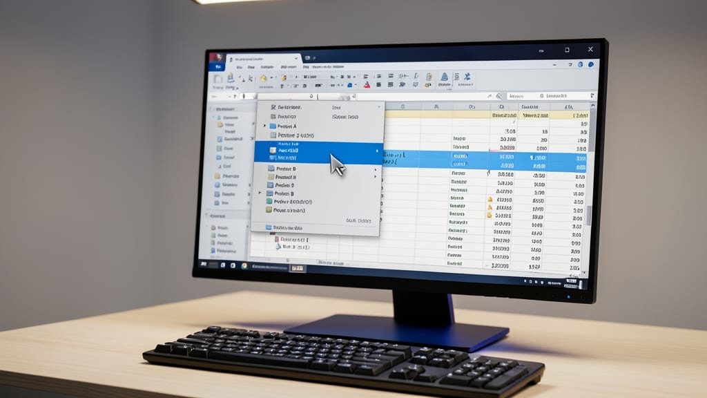
Tired of static dropdown menus that break when your data moves? INDIRECT and OFFSET let you create self-updating lookup tables without hardcoding cell references. This dynamic duo pulls data on-the-fly, making your spreadsheets adapt automatically to changes—ideal for inventory lists, product catalogs, or any scenario where data shifts frequently.

INDIRECT converts text strings into cell references (e.g., =INDIRECT("A"&ROW())), while OFFSET shifts ranges dynamically (e.g., =OFFSET(A1,1,0) moves down one row). Combined, they power flexible data validation lists that pull from hidden tables, ensuring dropdowns always reflect the latest data. Perfect for dashboards where ranges expand or contract.

Account managers tracking client lists or retailers updating product categories will love this—no more manual adjustments when data grows. Just set it up once, and your formulas stay future-proof. ✨

Tired of manually copying PivotTable values into reports? The GETPIVOTDATA function lets you pull exact metrics directly into cells—no dragging, no retyping, and no risk of errors from manual entry.

Simply reference your PivotTable with GETPIVOTDATA("field_name", PivotTableRange, "criteria1", "value1"), and Excel returns the precise value you need. This works seamlessly with dynamic ranges, so your reports stay updated automatically when the source data changes. Perfect for pulling quarterly sales figures, budget variances, or customer metrics into dashboards without rebuilding the table.

Accountants, analysts, and business owners will love this for error-free reporting—no more guessing which PivotTable version contains the latest data. ✨